Chapter 5
RL, RLC and AC Circuits
5.1 RL circuits
Recall that a changing current through an inductor induces a voltage that opposes the change, \(\mathcal E_L = -L\,dI/dt\) (3.6), where the inductance \(L\) depends only on geometry.
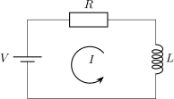
Consider a voltage source \(V\), a resistor \(R\) and an inductor \(L\) in series. Because of the definition of inductance, the inductor contributes \(\mathcal E_L = -L\,dI/dt\) to the loop rule: \[\begin{equation} \tag{5.1} \keyeq{\displaystyle V - IR - L\,\frac{dI}{dt} = 0} \end{equation}\]
This is the same equation as for the RC circuit, with \(Q\leftrightarrow I\). Recall (2.2), the loop rule \(V - IR - Q/C = 0\) with \(I = dQ/dt\): \[V - \frac{Q}{C} - R\,\frac{dQ}{dt} = 0, \qquad Q(t) = VC\left(1 - e^{-t/RC}\right).\] Under the replacements \[Q \to I, \qquad R \to L, \qquad C = \frac{1}{R}\] this becomes (5.1), so \[\keyeq{\displaystyle I(t) = \frac{V}{R}\left(1 - e^{-(R/L)\,t}\right)}\]
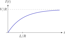
The time constant is \(L/R\) (compare \(RC\)). The inductor opposes changes in the current: \(I\) does not jump to \(V/R\) but grows gradually.
Connection with the oscillations chapter
We can also solve (5.1) with the strategy of the Oscillations chapter. The homogeneous equation \(L\,dI/dt + RI = 0\) is solved by guessing \(I = I_0\,e^{\lambda t}\), which gives \(\lambda = -R/L\). A constant \(I = V/R\) solves the full equation, so \(I(t) = V/R + I_0\,e^{-(R/L)t}\), and \(I(0) = 0\) fixes \(I_0 = -V/R\): the same result. This split into a homogeneous and a particular solution reappears for the driven RLC circuit below.
5.2 LC circuits
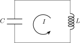
With no source, the loop rule is \(-L\,dI/dt - Q/C = 0\). Using \(I = dQ/dt\), \[\begin{equation} \tag{5.2} \keyeq{\displaystyle \frac{d^2Q}{dt^2} = -\frac{Q}{LC}} \end{equation}\] This is a harmonic oscillator!
Compare (4.1): \(Q\) plays the role of \(x\) and \(1/LC\) the role of \(k/m\). By (4.4), \[\keyeq{\displaystyle Q(t) = Q_0\cos(\omega t + \phi)}\;, \qquad \keyeq{\displaystyle \omega = \frac{1}{\sqrt{LC}}}\] where \(\omega\) is the natural angular frequency of the circuit.
5.3 RLC circuits
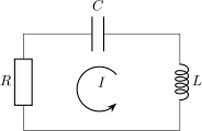
Adding a resistor to the LC circuit, the loop rule becomes \[\begin{equation} \tag{5.3} \keyeq{\displaystyle \frac{d^2Q}{dt^2} + \frac{R}{L}\,\frac{dQ}{dt} + \frac{Q}{LC} = 0} \end{equation}\] This is a damped oscillator!
Connection with the damped oscillator
Recall (4.5), \(m\,\ddot x + b\,\dot x + kx = 0\). Equation (5.3) is the same equation with \[m = 1, \qquad b = \frac{R}{L}, \qquad k = \frac{1}{LC}, \qquad x \leftrightarrow Q .\] (Multiplying (5.3) by \(L\) gives the equivalent dictionary: inductance \(\leftrightarrow\) mass, resistance \(\leftrightarrow\) damping coefficient \(b\), \(1/C \leftrightarrow\) spring constant \(k\).) The decay time \(\tau = 2m/b\) becomes \(2L/R\), and \(\omega_0 = \sqrt{k/m}\) becomes the LC frequency \(1/\sqrt{LC}\).
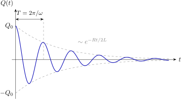
The solution of the damped oscillator then gives, in the underdamped case \(1/LC > (R/2L)^2\), \[\keyeq{\displaystyle Q(t) = Q_0\,e^{-(R/2L)\,t}\cos(\omega t + \phi)}\] with \[\keyeq{\displaystyle \omega = \sqrt{\frac{1}{LC} - \left(\frac{R}{2L}\right)^2}}\;, \qquad T = \frac{2\pi}{\omega} .\]
5.4 Driven RLC circuit
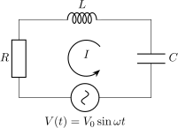
Now add a source \(V(t) = V_0\sin\omega t\). The loop rule (K2) gives \[\begin{equation} \tag{5.4} \keyeq{\displaystyle V_0\sin\omega t - L\,\frac{d^2Q}{dt^2} - R\,\frac{dQ}{dt} - \frac{Q}{C} = 0} \end{equation}\]
Strategy: homogeneous plus particular solution
Solve for \(Q = Q_h + Q_p\) (the general solution). The homogeneous part \(Q_h\) solves the equation without the source, \(L\ddot Q_h + R\dot Q_h + Q_h/C = 0\), so by the previous section \[Q_h(t) = Q_0\,e^{-(R/2L)\,t}\cos(\omega' t + \phi), \qquad \omega' = \sqrt{\frac{1}{LC} - \left(\frac{R}{2L}\right)^2}.\] This decays exponentially, so at late times only the particular solution \(Q_p\) remains.
Finding \(Q_p\)
Guess a response at the driving frequency, \[Q_p = \frac{A}{\omega}\cos\omega t + \frac{B}{\omega}\sin\omega t .\] Then the current we are looking for is \[I_p = \frac{dQ_p}{dt} = -A\sin\omega t + B\cos\omega t, \qquad \frac{d^2Q_p}{dt^2} = -A\omega\cos\omega t - \omega B\sin\omega t .\] Plugging into (5.4) gives \[\begin{align*} V_0\sin\omega t &= L\left(-A\omega\cos\omega t - B\omega\sin\omega t\right) \\ &\quad + R\left(-A\sin\omega t + B\cos\omega t\right) \\ &\quad + \frac{1}{\omega C}\left(A\cos\omega t + B\sin\omega t\right) \end{align*}\] Define \[R_{LC} := \omega L - \frac{1}{\omega C} .\] Matching the terms in \(\cos\omega t\): \[-L\omega A + RB + \frac{1}{\omega C}A = 0 \;\Longleftrightarrow\; -R_{LC}A + RB = 0 \;\Longrightarrow\; \keyeq{\displaystyle A = \frac{R}{R_{LC}}\,B}\] and in \(\sin\omega t\): \[-L\omega B - RA + \frac{1}{\omega C}B = V_0 \;\Longleftrightarrow\; -R_{LC}B - RA = V_0 \;\Longrightarrow\; \left(R_{LC} + \frac{R^2}{R_{LC}}\right)B = -V_0 .\] Hence \[\keyeq{\displaystyle B = -V_0\,\frac{R_{LC}}{R_{LC}^2 + R^2}} \qquad \keyeq{\displaystyle A = -V_0\,\frac{R}{R_{LC}^2 + R^2}}\]
Amplitude and phase of the current
The particular current \(I_p = B\cos\omega t - A\sin\omega t\) has the form \(C\cos\omega t + D\sin\omega t\) of the Oscillations chapter, so by (4.4) \[I_p(t) = I_0\cos(\omega t + \phi), \qquad I_0 = \sqrt{A^2 + B^2}, \qquad \tan\phi = \frac{A}{B}.\]
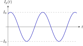
The current oscillates at the driving frequency \(\omega\), with the amplitude \(I_0\) found next.
Substituting \(A\) and \(B\), \[\keyeq{\displaystyle I_0 = V_0\sqrt{\frac{R_{LC}^2 + R^2}{\left(R_{LC}^2 + R^2\right)^2}} = \frac{V_0}{\sqrt{R_{LC}^2 + R^2}}}\]
Equivalently \(I_0 = V_0/R_{\mathrm{eff}}\) with the effective resistance \[R_{\mathrm{eff}} = \sqrt{\left(\omega L - \frac{1}{\omega C}\right)^2 + R^2} .\]
Resonance
The amplitude \(I_0\) is largest when \(R_{LC} = \omega L - 1/(\omega C) = 0\), that is at \[\keyeq{\displaystyle \omega_0 = \frac{1}{\sqrt{LC}}}\] the natural frequency of the LC circuit, where \(I_0 = V_0/R\). This is resonance!
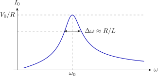
The width of the resonance peak is \(\Delta\omega \approx R/L\): the smaller the resistance, the sharper the peak.
Quality factor
The quality factor \(\mathsf{Q}\) (not to be confused with the charge \(Q\)) measures how narrow the resonance is, \[\keyeq{\displaystyle \mathsf{Q} = \frac{\omega_0}{\Delta\omega}}\] where \(\Delta\omega\) is the width of the peak between the points where the dissipated power (\(\propto I_0^2\)) has dropped to half its maximum, i.e. where \(I_0 = I_{\max}/\sqrt2\), equivalently \(|R_{LC}| = R\). When the peak is narrow (small \(R\)), we can expand around \(\omega_0\): \[R_{LC} = \frac{L\left(\omega^2 - \omega_0^2\right)}{\omega} \approx 2L\,(\omega - \omega_0),\] so \(|R_{LC}| = R\) at \(|\omega - \omega_0| = R/2L\), a full width \(\Delta\omega \approx R/L\). Therefore \[\keyeq{\displaystyle \mathsf{Q} \approx \frac{\omega_0 L}{R} = \frac{1}{R}\sqrt{\frac{L}{C}}}\] Using \(\tau = 2L/R\) from the damped oscillator, this is also \(\mathsf{Q}\approx\omega_0\tau/2\): a large \(\mathsf Q\) means weak damping and a sharp resonance.
Problems
Problems are taken from the sources listed under Sources and Attribution. Numbers refer to the end-of-chapter problems; figures have been redrawn.
OpenStax University Physics Vol. 2, Chapter 14: Inductance
14.53
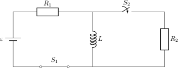
For the circuit shown, \(\varepsilon = 20\,\mathrm{V}\), \(L = 4.0\,\mathrm{mH}\), and \(R = 5.0\,\mathrm{\Omega }\). After steady state is reached with \(S_1\) closed and \(S_2\) open, \(S_2\) is closed and immediately thereafter (at \(t=0\)) \(S_1\) is opened. Determine (a) the current through \(L\) at \(t=0\), (b) the current through \(L\) at \(t=4.0\times 10^{-4}\,\mathrm{s}\), and (c) the voltages across \(L\) and \(R_2\) at \(t=4.0\times 10^{-4}\,\mathrm{s}\). \(R_1 = R_2 = R\).
14.65
In an oscillating LC circuit, the maximum charge on the capacitor is \(2.0\times 10^{-6}\,\mathrm{C}\) and the maximum current through the inductor is \(8.0\,\mathrm{mA}\). (a) What is the period of the oscillations? (b) How much time elapses between an instant when the capacitor is uncharged and the next instant when it is fully charged?
14.71
In an oscillating RLC circuit with \(L=10\,\mathrm{mH}\), \(C=1.5\,\mathrm{\mu F}\), and \(R=2.0\,\mathrm{\Omega }\), how much time elapses before the amplitude of the oscillations drops to half its initial value?
OpenStax University Physics Vol. 2, Chapter 15: Alternating-Current Circuits
15.39
For an RLC series circuit, \(R=100\,\mathrm{\Omega }\), \(L=150\,\mathrm{mH}\), and \(C=0.25\,\mathrm{\mu F}\). (a) If an ac source of variable frequency is connected to the circuit, at what frequency is maximum power dissipated in the resistor? (b) What is the quality factor of the circuit?
15.41
(a) What is the resonant frequency of a resistor, capacitor, and inductor connected in series if \(R=100\,\mathrm{\Omega }\), \(L=2.0\,\mathrm{H}\), and \(C=5.0\,\mathrm{\mu F}\)? (c) What is the Q of the circuit? (d) What is the bandwidth of the circuit?