Lab 2 Formative
Inductance and Internal Resistance
Before the lab, read the Background section below and answer Question 1. The error propagation rules you will need are in the Lab Guide.
L2.1 Goals
Study the growth/decay curves of an RL circuit.
Estimate the internal resistance of a waveform generator using the rated value of the inductance \(L\) and the growth/decay curves of an RL circuit.
Gain confidence in the oscilloscope fall/rise-time method introduced in Lab 1 by applying it to a new circuit.
Practice propagating errors through a calculation (see Error propagation in the Lab Guide).
Familiarize yourselves with the use of inductors and the limitations of “ideal” circuit components.
L2.2 Background
Measuring inductance and internal resistance
In Lab 1, we measured the capacitance \(C\) of a capacitor by placing it in series with a resistor of resistance \(R\) and measuring the time constant \(\tau_\text{RC} = RC\). We did this by using a wave generator to drive the circuit with a square wave, and by using the oscilloscope to measure the fall time \(\Delta t\) of the voltage across the resistor between 80% and 20% of its maximum value. Using the theoretical form of this curve, we found (Question 1 of Lab 1) that \(\tau_\text{RC}\) could be determined from \(\Delta t\). Knowing \(R\) from a multimeter measurement then gave us \(C\).
In this experiment, we will use a similar setup. This time, however, we will use an RL circuit to measure the internal resistance of the wave generator, using the rated value of the inductance \(L\) of the inductor.
Just as before, we will use the wave generator to apply a square-wave voltage to the circuit, and record the voltage across the resistor during the charge and discharge cycles using the oscilloscope. Now, however, the current through the resistor rises when the voltage steps up (see the RL circuit, (5.1), in RL, RLC and AC Circuits). The voltage is \[\begin{equation} \tag{L2.1} V_\text{R}(t) = V_0\left(1 - e^{-Rt/L}\right), \end{equation}\] so that the time constant is \[\begin{equation} \tag{L2.2} \keyeq{\displaystyle \tau_\text{RL} = \frac{L}{R}} \end{equation}\] By measuring the rise time \(\Delta t\), the time it takes for the voltage to rise from 20% to 80% of its maximum value, we can determine \(\tau_\text{RL}\) and then compute \(R\) using the rated value of \(L\).
Question 1: Compute \(\tau_\text{RL}\) from the rise time \(\Delta t\). How does your answer compare to the relation between \(\tau_\text{RC}\) and \(\Delta t\) that you found in Lab 1? Insert your answer below.
\(\tau_\text{RL} = {}\)
Because \(R\) appears in the denominator of (L2.2), a large value of \(R\) makes \(\tau_\text{RL}\) very short. Since commercially available inductors usually have \(L\) in the millihenry range, we need to keep \(R\) as small as possible so that \(\tau_\text{RL}\) stays within a reasonable range for our scope.
Unfortunately, this means that the total resistance of the circuit is dominated not by the resistor itself but by the internal resistance of the wave generator. This resistance is set to around \(600\,\mathrm{\Omega }\) but is not known exactly, and it is already large enough to make \(\tau_\text{RL}\) fairly small. (It was also present in the RC circuit of Lab 1, but was negligible next to the \(100\,\mathrm{k\Omega }\) resistor.) Because the inductor itself also has some resistance, the total resistance of the circuit is \[\begin{equation} \tag{L2.3} \keyeq{R = R_R + R_L + R_\text{int}} \end{equation}\] where \(R_R\) is the resistance of the resistor, \(R_L\) the (DC) resistance of the inductor, and \(R_\text{int}\) the internal resistance of the wave generator.
In this experiment, we will determine \(R_\text{int}\) by first finding \(\tau_\text{RL}\) from a measurement of \(\Delta t\), and then measuring \(R_R\) and \(R_L\).
L2.3 Materials
Multimeter
Oscilloscope (\(10\,\mathrm{MHz}\) Picoscope 2204A with accompanying software) and two probes
Wave generator
Breadboard
Resistor (rated \(100\,\mathrm{\Omega }\))
Inductors (rated \(2.7\,\mathrm{mH}\) and \(1.0\,\mathrm{mH}\))
Wires
L2.4 Instructions
Measure the DC resistance of the \(100\,\mathrm{\Omega }\) resistor and of the \(2.7\,\mathrm{mH}\) inductor using a multimeter. Record the minimum resolution of the meter reading to estimate the error.
Resistance measurements
Resistor resistance (\(R_R\)): \(\pm\) \(\mathrm{\Omega }\) (measured with multimeter)
Inductor resistance (\(R_L\)): \(\pm\) \(\mathrm{\Omega }\) (measured with multimeter)
Record the rated value of the inductance and its tolerance (ask the instructor if the tolerance is not given). This gives an estimate of the error in \(L\).
Inductor rating
Rated inductance (\(L\)): \(\pm\) \(\mathrm{mH}\) (rated value and tolerance)
Set up the series RL circuit of Figure L2.1 as shown in Figure L2.2.
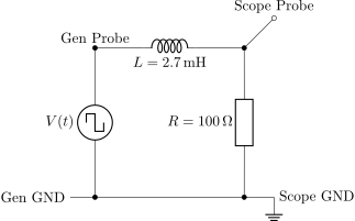
Figure L2.1. RL circuit driven by a square-wave generator. The oscilloscope measures the voltage across the resistor (between Scope Probe and Scope GND).
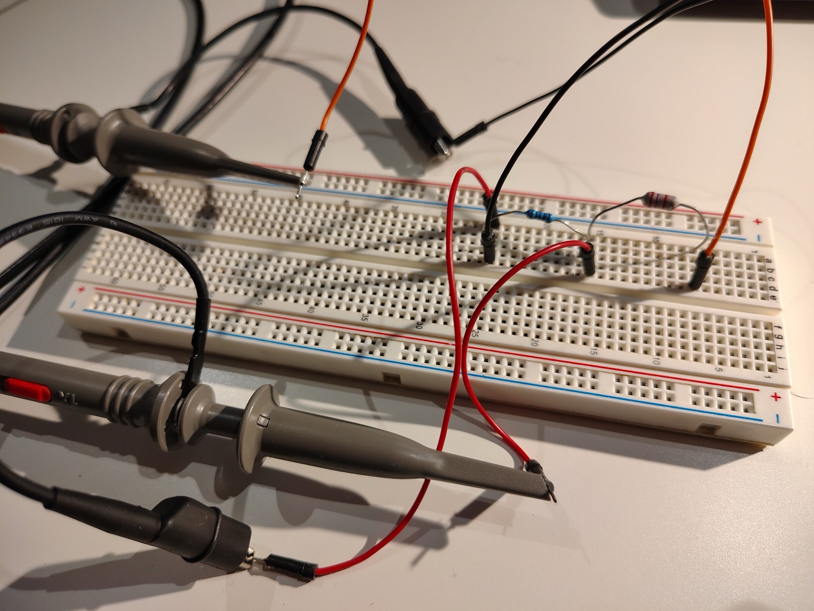
Estimate \(\tau_\text{RL}\) from (L2.2) and (L2.3), using the measured values of \(R_R\) and \(R_L\) and the rough rated value \(R_\text{int} \approx 600\,\mathrm{\Omega }\). Use this to choose reasonable settings for the scope timescale and the generator frequency (see Question 3 of Lab 1 for how to choose these). You may also need to change the maximum voltage scale and the trigger settings.
Time constant estimate
\(\tau_\text{RL, estimate}\): \(\mathrm{\mu s}\)
Using the software’s measurement tools, measure the rise time \(\Delta t\) and its standard deviation \(\sigma\) over many cycles (\(n > 100\)).
Rise time measurement (\(2.7\,\mathrm{mH}\))
Rise time (\(\Delta t\)): \(\pm\) \(\mathrm{\mu s}\) (from oscilloscope measurements)
Standard deviation (\(\sigma\)): \(\mathrm{\mu s}\)
Repeat for the \(1.0\,\mathrm{mH}\) inductor if there is time. Remember to measure its DC resistance first!
Rise time measurement (\(1.0\,\mathrm{mH}\))
Inductor resistance (\(R_L\)): \(\pm\) \(\mathrm{\Omega }\) (measured with multimeter)
Rise time (\(\Delta t\)): \(\pm\) \(\mathrm{\mu s}\) (from oscilloscope measurements)
Standard deviation (\(\sigma\)): \(\mathrm{\mu s}\)
L2.5 Analysis
Show your derivations for all calculations. Every number you report should come with an error! When computing an error for a derived quantity, use the rules in Error propagation in the Lab Guide. The natural places to propagate errors in this lab are marked below.
Compute \(\tau_\text{RL}\) from the measured rise time \(\Delta t\) using your answer to Question 1. Propagate the error in \(\Delta t\) (which you can estimate from \(\sigma\)) to find the error in \(\tau_\text{RL}\). Hint: the factor relating \(\Delta t\) and \(\tau_\text{RL}\) is an exact number with no error. What does the multiplication/division rule (L0.2) say about the relative error in this case?
Compute the total resistance \(R\) of the circuit using (L2.2) and the rated value of \(L\). Propagate the errors in \(\tau_\text{RL}\) and in \(L\) (from its tolerance) to find the error in \(R\).
Compute the measured value of \(R_\text{int}\) using (L2.3). Propagate the errors in \(R\), \(R_R\) and \(R_L\) (from the multimeter resolution) to find the error in \(R_\text{int}\). Compare your result to the rough rated value of \(600\,\mathrm{\Omega }\). Are they consistent within your error?
Which of the errors above contributes most to the error in \(R_\text{int}\)? How could the experiment be improved to reduce it?
If you measured both inductors, repeat the calculation above for the \(1.0\,\mathrm{mH}\) inductor. Compute the difference between the two values of \(R_\text{int}\) and propagate the errors to find its error. Is the difference consistent with zero? What does this tell you about the reliability of the method?
What other sources of systematic error are there in this measurement that are not captured by the error estimates above? (Hint: how does the rise time of the generator’s square wave itself compare to \(\Delta t\)?)
Keep a record of these results. You will use them for the Signals Lab!