Lab 1 Formative
Resistance and Capacitance
Before the lab, read the Lab Guide (general instructions and error propagation) and the Background section below, and answer Question 1.
L1.1 Goals
Measure the resistance of resistors in series and in parallel and verify the theoretical predictions.
Accurately measure the capacitance of a capacitor indirectly, using the growth/decay curves of an RC circuit.
Familiarize yourselves with the setup and operation of an oscilloscope.
Familiarize yourselves with the scope’s software and analysis tools.
Familiarize yourselves with the use of breadboards and basic circuit components such as capacitors and resistors.
(Optional) Measure the capacitance of capacitors in series and in parallel and verify the theoretical predictions.
L1.2 Background
Resistance and capacitance in series and parallel
The effective resistance of resistors in series, \(R_s\), and in parallel, \(R_\parallel\), is \[\begin{equation} \tag{L1.1} \begin{aligned} R_s &= R_1 + R_2 + \dots \\ \frac{1}{R_\parallel} &= \frac{1}{R_1} + \frac{1}{R_2} + \dots , \end{aligned} \end{equation}\] where \(R_i\) is the resistance of the \(i\)-th resistor. Similarly, for capacitors, \[\begin{equation} \tag{L1.2} \begin{aligned} \frac{1}{C_s} &= \frac{1}{C_1} + \frac{1}{C_2} + \dots \\ C_\parallel &= C_1 + C_2 + \dots . \end{aligned} \end{equation}\]
Measuring capacitance
While resistance can be measured directly using a multimeter, capacitance cannot: \(C = Q/V\), and the charge \(Q\) on the plates cannot be measured directly. Capacitance can, however, be measured indirectly by determining the characteristic charge/discharge time \(\tau_\text{RC} = RC\) of an RC circuit. Knowing \(R\) then gives \[\begin{equation} \tag{L1.3} \keyeq{\displaystyle C = \frac{\tau_\text{RC}}{R}} \end{equation}\] In class (Current, Resistance & DC Circuits), we found that the voltage across the capacitor of an RC circuit is \[\begin{equation} \tag{L1.4} \begin{aligned} V_\text{C,charge}(t) &= V_0\left(1 - e^{-t/RC}\right) \\ V_\text{C,discharge}(t) &= V_0\,e^{-t/RC} . \end{aligned} \end{equation}\] In this experiment, we will build an RC circuit and use it to measure \(C\) indirectly.
To do this, we will use a wave generator to produce a square wave that drives the RC circuit. This alternates the voltage between \(-V_0\) and \(V_0\) at regular intervals, so that the capacitor is alternately charged and discharged. We will then use an oscilloscope probe to measure the voltage across the resistor. Since the current through the circuit is \(I = C\,dV_\text{C}/dt\), the voltage across the resistor is found by taking the derivative of the charging curve in (L1.4) and multiplying by \(RC\): \[\begin{equation} \tag{L1.5} \keyeq{V_\text{R}(t) = V_0\,e^{-t/RC}} \end{equation}\]
We will use the software provided with the oscilloscope to measure the fall time: the time it takes for the voltage to fall from 80% to 20% of its maximum value. Call this time \(\Delta t\). Note that it does not depend on \(V_0\), so we do not need to know the exact amplitude of the signal delivered to the circuit.
Question 1: Using (L1.5), compute \(\tau_\text{RC}\) from the fall time \(\Delta t\). Insert your answer below.
\(\tau_\text{RC} = {}\)
L1.3 Materials
Multimeter
Oscilloscope (\(10\,\mathrm{MHz}\) Picoscope 2204A with accompanying software) and two probes
Wave generator
Breadboard
Capacitors (rated \(15\,\mathrm{n F}\) and \(100\,\mathrm{n F}\))
Resistors (two rated \(2\,\mathrm{k\Omega }\) and one rated \(100\,\mathrm{k\Omega }\))
Wires
L1.4 Instructions
Resistors in series and parallel
Use the multimeter to measure and record the resistance of the two \(2\,\mathrm{k\Omega }\) resistors and of the \(100\,\mathrm{k\Omega }\) resistor. Record the minimum resolution of the meter reading: this gives an estimate of the error in the resistance. Note that the actual resistance may differ from its rated value.
Resistance measurements
First \(2\,\mathrm{k\Omega }\) resistor (\(R_1\)): \(\pm\) \(\mathrm{k\Omega }\) (measured with multimeter)
Second \(2\,\mathrm{k\Omega }\) resistor (\(R_2\)): \(\pm\) \(\mathrm{k\Omega }\) (measured with multimeter)
\(100\,\mathrm{k\Omega }\) resistor (\(R_R\)): \(\pm\) \(\mathrm{k\Omega }\) (measured with multimeter)
Arrange the two \(2\,\mathrm{k\Omega }\) resistors in series and in parallel on the breadboard and measure their effective resistance using the multimeter. Compare the measured values with theory.
Series and parallel resistance
Series resistance (\(R_s\)): \(\pm\) \(\mathrm{k\Omega }\) (measured with multimeter)
Parallel resistance (\(R_\parallel\)): \(\pm\) \(\mathrm{k\Omega }\) (measured with multimeter)
Question 2: Using (L1.1), predict the series and parallel resistance of the two \(2\,\mathrm{k\Omega }\) resistors. Are the predicted values distinguishable from the rated value of a single resistor, given the resolution of the multimeter?
Measuring capacitance
Set up the series RC circuit of Figure L1.1 as shown in Figure L1.2. Use the \(100\,\mathrm{k\Omega }\) resistor and the \(15\,\mathrm{n F}\) capacitor, and note the capacitor’s rating.
Capacitor rating
Capacitor rating (\(C_\text{rating}\)): \(\mathrm{n F}\)
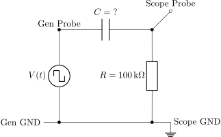
Figure L1.1. RC circuit driven by a square-wave generator. The oscilloscope measures the voltage across the resistor (between Scope Probe and Scope GND).
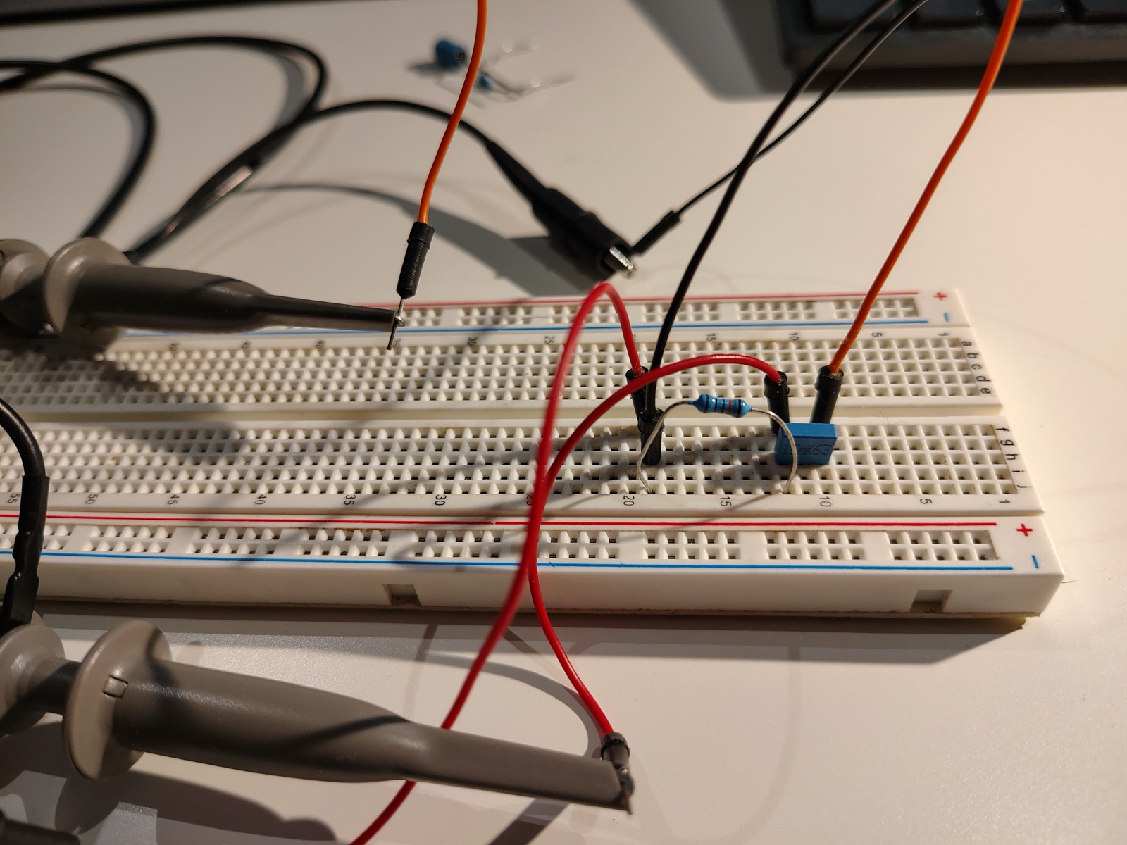
Use the measured value of \(R\) and the rated value of \(C\) to estimate \(\tau_\text{RC}\).
Time constant estimate
\(\tau_\text{RC, estimate}\): \(\mathrm{ms}\)
Using the Picoscope software, set the timescale on the scope to \(2\,\mathrm{ms}\)/div, the voltage scale to a maximum of \(2\,\mathrm{V}\), and the trigger to auto (you may later need to adjust the trigger level manually to get a stable signal).
Set the waveform generator to the square-wave setting, with a frequency between \(50\,\mathrm{Hz}\) and \(70\,\mathrm{Hz}\).
Question 3: Why are these good timescale and frequency settings?
Once you have a clear signal, use the “measurements” button to measure the fall time over many cycles (\(n > 100\)). Note the value of \(\sigma\), the standard deviation of the measurement, which is useful for estimating the random error.
Fall time measurement (\(15\,\mathrm{n F}\))
Fall time (\(\Delta t\)): \(\pm\) \(\mathrm{ms}\) (from oscilloscope measurements)
Standard deviation (\(\sigma\)): \(\mathrm{ms}\)
Repeat the measurement with the \(100\,\mathrm{n F}\) capacitor. You will need to re-estimate \(\tau_\text{RC}\) and change the scope timescale and generator frequency accordingly (see Question 3).
Fall time measurement (\(100\,\mathrm{n F}\))
Fall time (\(\Delta t\)): \(\pm\) \(\mathrm{ms}\) (from oscilloscope measurements)
Standard deviation (\(\sigma\)): \(\mathrm{ms}\)
(Optional, if time allows.) Place the two capacitors in series and then in parallel, and repeat the measurement for each combination. Remember to estimate \(\tau_\text{RC}\) first to choose reasonable scope and generator settings.
Capacitors in series and parallel
Series fall time (\(\Delta t_s\)): \(\pm\) \(\mathrm{ms}\) (from oscilloscope measurements)
Parallel fall time (\(\Delta t_\parallel\)): \(\pm\) \(\mathrm{ms}\) (from oscilloscope measurements)
L1.5 Analysis
Do your results confirm or refute the formulas (L1.1) for resistance in series and in parallel?
Compute the measured value of \(C\) for each capacitor using the measured value of \(\Delta t\), your answer to Question 1, and (L1.3). Compare this to its rated value.
Estimate the error in these measurements using \(\sigma\) and your error estimate for \(R\) (see Error propagation in the Lab Guide).
(Optional) Do your results for the capacitors in series and parallel confirm or refute the formulas (L1.2) for capacitance? Compare to the values predicted using your measured values of \(C\).
What are possible sources of systematic error in this measurement? (Hint: the input resistance of the scope is \(1\,\mathrm{M\Omega }\). How does this compare to \(R\), and how does the scope probe connect to the circuit? What about the internal resistance of the wave generator, which is around \(600\,\mathrm{\Omega }\)?)
Keep a record of these results. You will use them in the next lab and in the Signals Lab!