Lab 3 Summative
Signals Lab: RLC Circuits
This is the summative lab: it is assessed by a lab report (see the instructions at the end). Before the lab, read the Background section below. The error propagation rules you will need are in the Lab Guide, and you will use your results from Lab 1 and Lab 2.
L3.1 Goals
Determine the (high-pass) response curve across the resistor of a series RC circuit, and use it to measure the capacitance.
Determine the (band-pass) response curve across the resistor of a series RLC circuit, and use it to measure the resistance and inductance.
Determine the ringdown curve of a charged series RLC circuit, and use it to measure the resistance and inductance.
Learn to estimate and evaluate random and systematic errors in different experimental setups.
L3.2 Background
RC circuits as high-pass filters
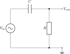
As we saw in class (Introduction to Signal Processing), a series RC circuit can function as a high-pass filter when the output is taken across the resistor. At low frequencies the capacitor acts effectively as an open circuit, and at high frequencies as a short circuit, allowing high-frequency signals to pass through to the resistor.
Recall from class that the response function \(h(\omega)\), which measures the amplitude attenuation of a pure sine wave with angular frequency \(\omega\), is \[\begin{equation} \tag{L3.1} \keyeq{\displaystyle h(\omega) = \frac{V_\text{out}}{V_\text{in}} = \frac{RC\omega}{\sqrt{1 + (RC\omega)^2}}} \end{equation}\] where \(V_\text{in}\) and \(V_\text{out}\) are the voltage amplitudes of the incoming and filtered sine waves. The cutoff angular frequency \(\omega_c\), defined by \(h(\omega_c) = 1/\sqrt 2\), is \[\begin{equation} \tag{L3.2} \omega_c = \frac{1}{RC} , \qquad\text{or, as a frequency,}\qquad f_c = \frac{1}{2\pi RC} . \end{equation}\] For frequencies much larger than \(f_c\), \(h \approx 1\) and the signal passes through unattenuated. For frequencies much smaller than \(f_c\), the signal drops linearly with frequency: \(h(\omega) \approx RC\omega = \omega/\omega_c = f/f_c\). Figure L3.1 shows this behaviour for values of \(R\) and \(C\) similar (but not identical) to those we will encounter in this lab.
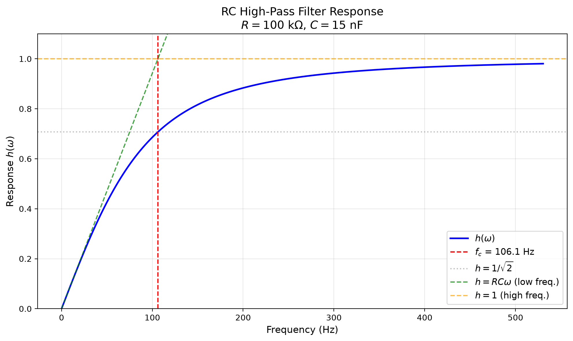
Figure L3.1. Frequency response of the RC high-pass filter, \(h(\omega)\) as a function of frequency, with the low-frequency asymptote \(h = RC\omega\) and the high-frequency asymptote \(h = 1\) for reference.
RLC circuits as band-pass filters
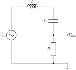
A series RLC circuit can function as a band-pass filter when the output is taken across the resistor. The inductor and capacitor form a resonant circuit that lets signals near the resonance frequency pass, while attenuating both low- and high-frequency signals.
Recall that we derived in class (the resonance curve of the driven RLC circuit) that the frequency response across the resistor of a series RLC circuit is \[\begin{equation} \tag{L3.3} \keyeq{\displaystyle h(\omega) = \frac{1}{\sqrt{\left(\dfrac{\omega^2 - \omega_0^2}{\omega\,\Delta\omega}\right)^2 + 1}}} \end{equation}\] where \(\omega_0\) is the resonant frequency and \(\Delta\omega\) is the full width at half maximum, or simply the bandwidth: \[\begin{equation} \tag{L3.4} \omega_0 = \frac{1}{\sqrt{LC}} , \qquad \Delta\omega = \frac{R}{L} . \end{equation}\] The two frequencies at which \(h = 1/\sqrt 2\) are separated by exactly \(\Delta\omega\); when \(\omega_0 \gg \Delta\omega\) they lie at \(\omega_0 \pm \frac12\Delta\omega\). The quality factor \[\begin{equation} \tag{L3.5} Q = \frac{\omega_0}{\Delta\omega} \end{equation}\] measures the sharpness of the peak: values much larger than 1 mean sharper peaks. When \(R\), \(L\) and \(C\) are tuned so that \(Q\) is large, the RLC circuit only lets a very narrow band of frequencies pass, and the circuit is said to “resonate” at those frequencies. Figure L3.2 shows this behaviour for parameters similar (but not identical) to those studied in this experiment. Note that the quality factor in this experiment is relatively small, \(Q \approx 1.9\), so the passband is relatively wide.
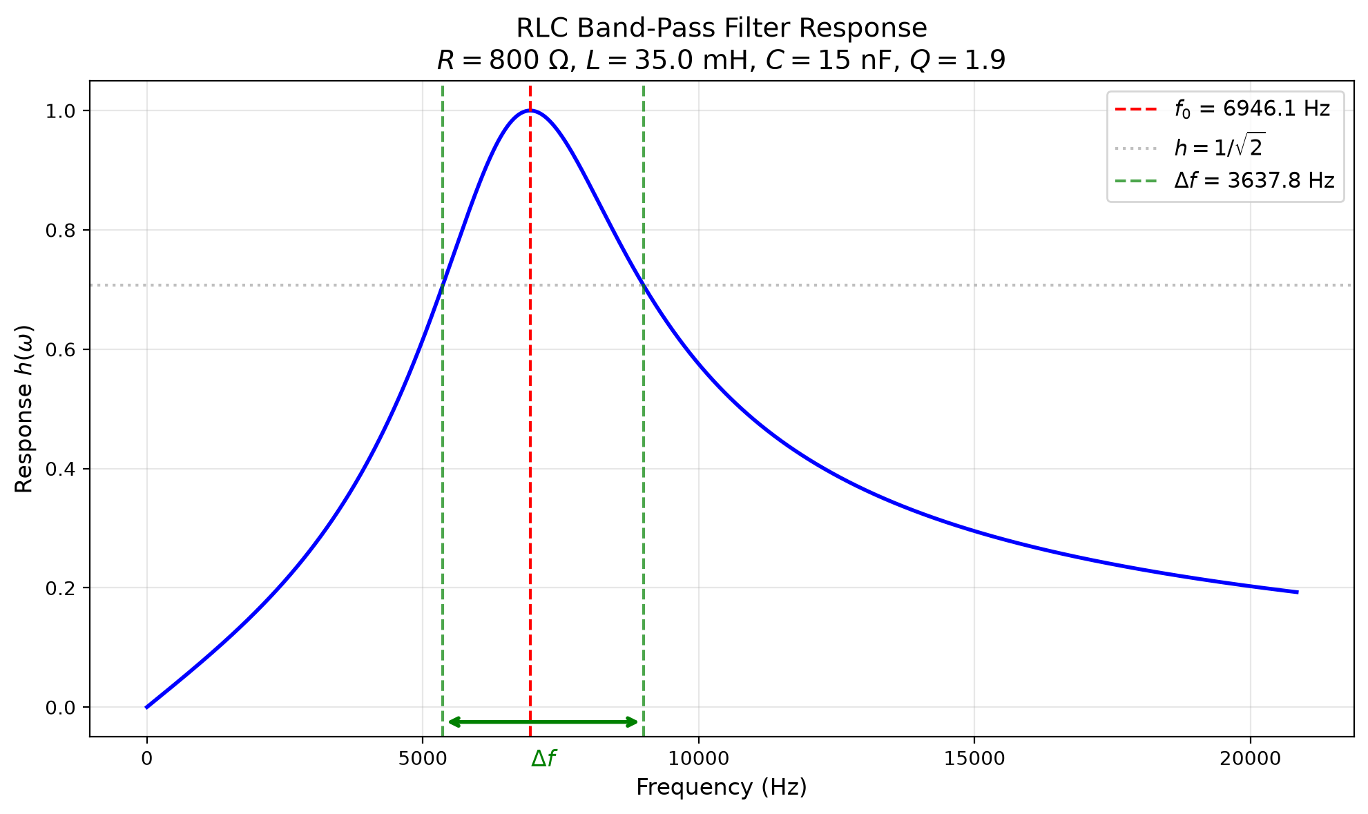
Figure L3.2. Frequency response of the RLC band-pass filter, \(h(\omega)\) as a function of frequency, with the resonance frequency \(f_0\) and the bandwidth \(\Delta f = \Delta\omega/2\pi\) marked.
Ringdown in an RLC circuit
In class (RL, RLC and AC Circuits), we studied what happens in an RLC circuit if the applied voltage is suddenly dropped to zero: the circuit becomes mathematically equivalent to a damped harmonic oscillator, (5.3). The voltage across the resistor is \[\begin{equation} \tag{L3.6} \keyeq{V_\text{out}(t) = V_0\,e^{-t/\tau}\sin(\omega' t - \phi)} \end{equation}\] where the decay time \(\tau\) and the ringdown frequency \(\omega'\) are \[\begin{equation} \tag{L3.7} \tau = \frac{2L}{R} , \qquad \omega' = \sqrt{\frac{1}{LC} - \left(\frac{R}{2L}\right)^2} = \sqrt{\omega_0^2 - \frac{1}{\tau^2}} . \end{equation}\] This formula holds provided \(\omega_0\tau = 2Q > 1\), which will be satisfied here. The parameters of (L3.6) are \(V_0\), which is determined by the initial voltage, and \(\phi\), which is determined by the initial rate of change, if any, of the voltage. We will set things up so that \(\phi = 0\).
In this experiment, we will use the wave generator to produce a sudden drop in the voltage using a step function, and use the oscilloscope probe to measure the voltage response across the resistor and verify (L3.6). We can measure the period \(T = 2\pi/\omega'\) of the oscillations by noting that the sine goes through zero at \(t = 0, \tfrac{T}{2}, T, \dots\). Since \(e^{-t/\tau} > 0\), \(V_\text{out}(t)\) in (L3.6) can only go through zero when the oscillating part does. So you can measure the period by noting where \(V_\text{out}\) goes through zero.
To find \(\tau\), we use the fact that the sine is periodic: \(\sin(\omega' t) = \sin\big(\omega'(t + T)\big)\). If we choose some time \(t_1\) (say, when the function is at a peak), the oscillating part has the same value at \(t = t_1 + T\); only the exponential \(e^{-t/\tau}\) has changed. Calling \(V_1 = V_\text{out}(t_1)\) and \(V_2 = V_\text{out}(t_1 + T)\), we see that \[\frac{V_1}{V_2} = e^{T/\tau} .\] Taking logarithms of both sides and rearranging gives \[\begin{equation} \tag{L3.8} \keyeq{\displaystyle \tau = \frac{T}{\ln(V_1/V_2)}} \end{equation}\] So by measuring \(V_1\) and \(V_2\), and using the measured value of \(T\), we can calculate \(\tau\). Figure L3.3 illustrates the procedure for values similar (but not identical) to those we will encounter in this experiment.
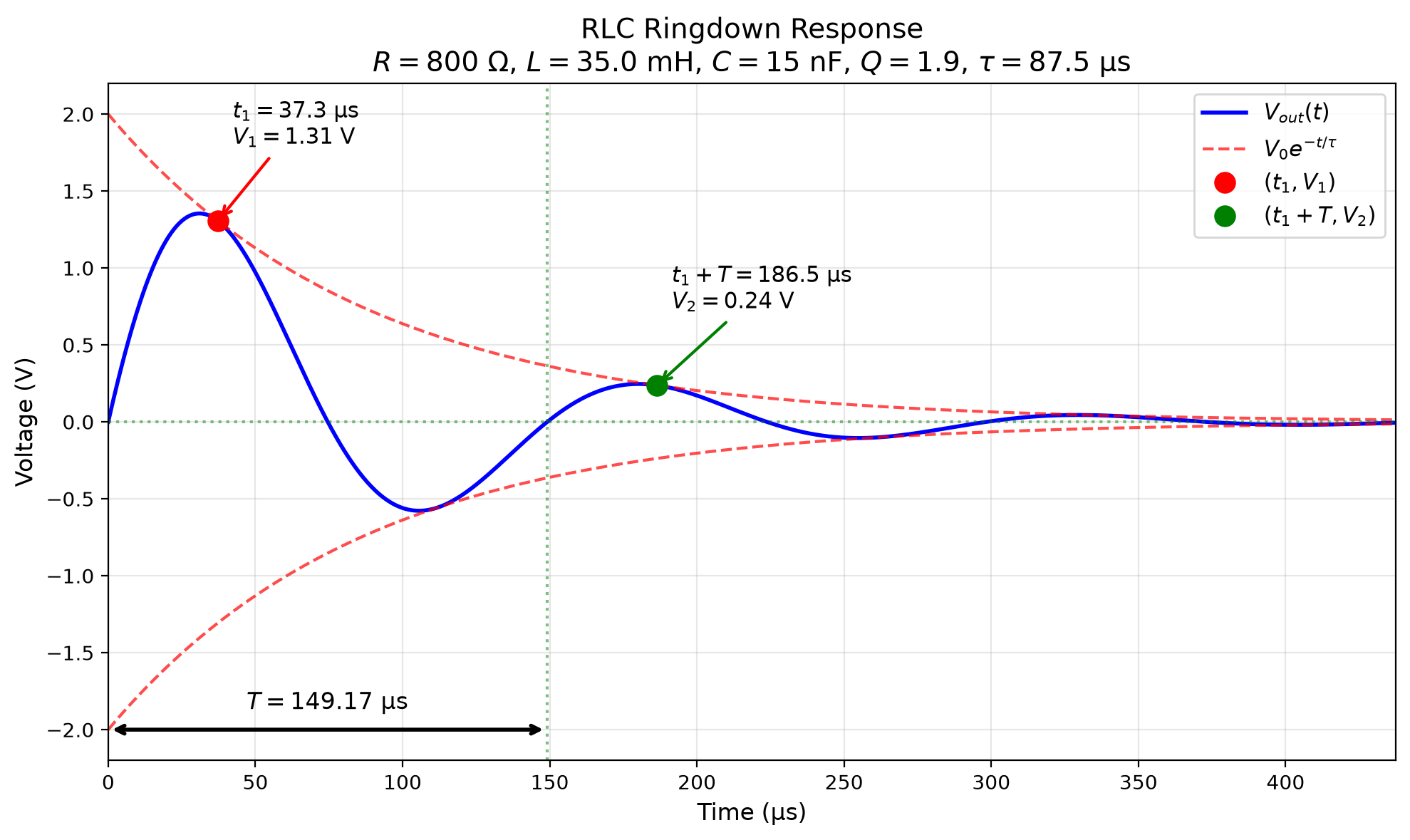
Figure L3.3. RLC ringdown after a step-function voltage drop. A peak \((t_1, V_1)\), the point \((t_1 + T, V_2)\) one period later, and the period \(T\) are marked. The red dashed lines show the exponential envelope \(V_0\,e^{-t/\tau}\).
Internal resistance
Just as in Lab 2, the wave generator has an internal resistance of about \(600\,\mathrm{\Omega }\), which is significant compared to the resistance \(R_R\) of the resistor and \(R_L\) of the inductor. The value of \(R\) in the RLC circuit is the sum of all three: \[\begin{equation} \tag{L3.9} R = R_R + R_L + R_\text{int} . \end{equation}\]
L3.3 Materials
Multimeter
Oscilloscope (\(10\,\mathrm{MHz}\) Picoscope 2204A with accompanying software) and two probes
Breadboard
Capacitor (rated \(15\,\mathrm{n F}\))
Resistors (rated \(100\,\mathrm{\Omega }\) and \(100\,\mathrm{k\Omega }\))
Inductor (unknown value)
Wires
L3.4 Instructions
RLC response curve
Use the multimeter to measure the exact resistance of the resistor rated \(100\,\mathrm{\Omega }\) and of the inductor. Note the minimum resolution of the multimeter reading: this gives an estimate of the error in the measured resistance.
Resistance measurements
Resistor resistance (\(R_R\)): \(\pm\) \(\mathrm{\Omega }\) (measured with multimeter)
Inductor resistance (\(R_L\)): \(\pm\) \(\mathrm{\Omega }\) (measured with multimeter)
Set up the series RLC band-pass circuit of the Background section as shown in Figure L3.4.
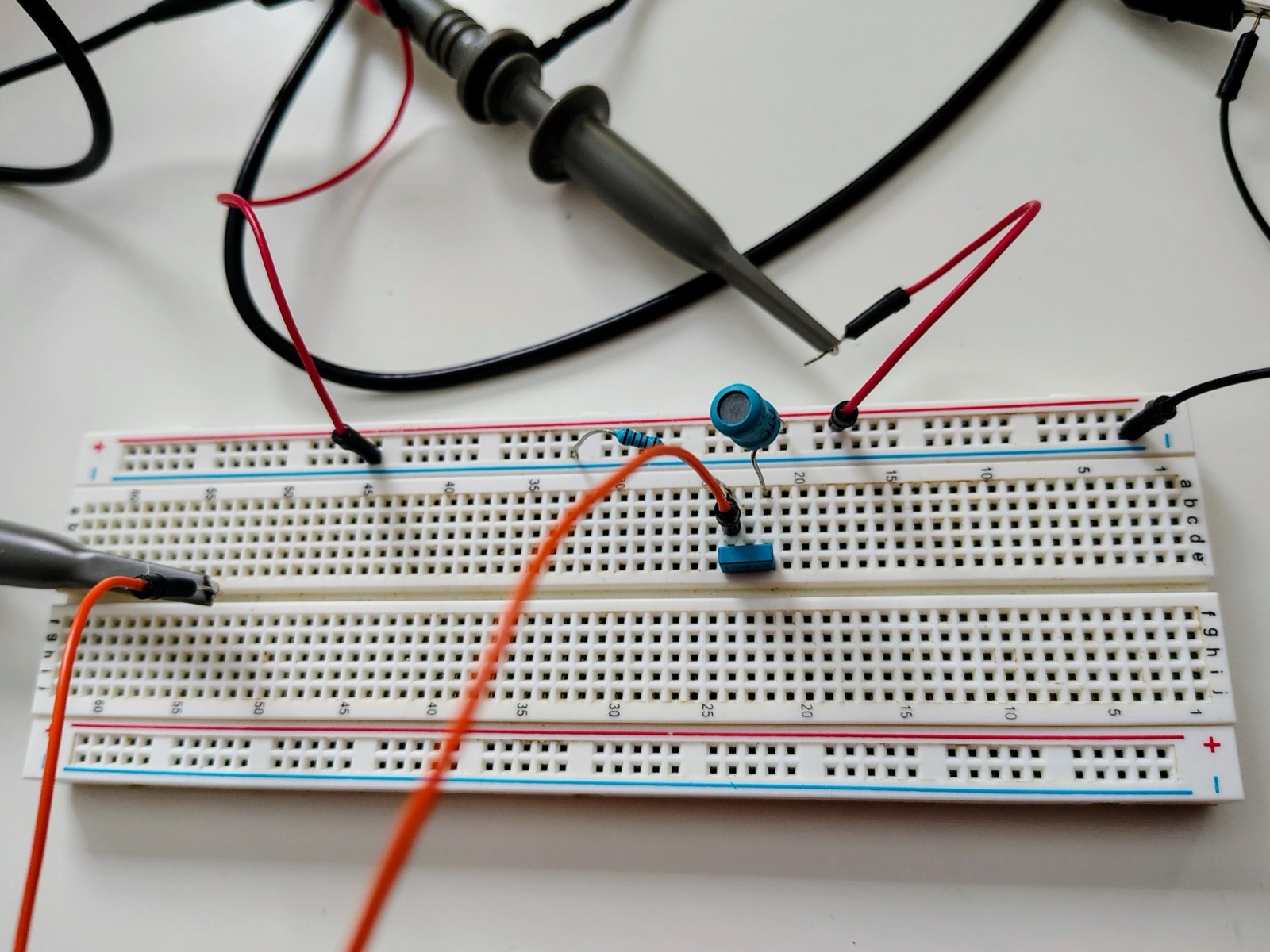
Figure L3.4. The series RLC band-pass circuit on a breadboard.
Using the Picoscope software, set the timescale on the scope to \(100\,\mathrm{\mu s}\)/div, the maximum voltage scale to \(500\,\mathrm{m V}\), and the trigger to auto (you may need to adjust it manually later to get a stable signal).
Set the waveform generator to the sine-wave setting and the amplitude to \(2\,\mathrm{V}\).
Scan the frequency in \(1\,\mathrm{kHz}\) steps from \(2\,\mathrm{kHz}\) to \(15\,\mathrm{kHz}\). Use the built-in “peak-to-peak” measurement of the Picoscope software to measure \(V_\text{out}\) as a function of frequency. (Note that the amplitude of \(V_\text{out}\) is half the peak-to-peak voltage.)
Record these readings in your notebook.
Focus on the peak of \(V_\text{out}\). Scan near the peak in \(0.1\,\mathrm{kHz}\) steps to find \(f_0\), and estimate the error of this measurement.
Resonance frequency
Resonance frequency (\(f_0\)): \(\pm\) \(\mathrm{kHz}\) (peak of response curve)
Do the same to find the frequencies \(f_\text{low}\) and \(f_\text{high}\) at which \(V_\text{out}\) is \(1/\sqrt 2\) of its maximum value. (Hint: use a horizontal ruler to find the right value of \(V_\text{out}\).) Use these to find the bandwidth \(\Delta f\).
Bandwidth measurements
Lower frequency (\(f_\text{low}\)): \(\pm\) \(\mathrm{kHz}\) (at \(1/\sqrt{2}\) of max amplitude)
Upper frequency (\(f_\text{high}\)): \(\pm\) \(\mathrm{kHz}\) (at \(1/\sqrt{2}\) of max amplitude)
Bandwidth (\(\Delta f\)): \(\pm\) \(\mathrm{kHz}\) (\(f_\text{high} - f_\text{low}\))
RLC ringdown
Set the Picoscope to \(V_\text{max} = \pm200\,\mathrm{m V}\) and the timescale to \(50\,\mathrm{\mu s}\)/div.
Set the generator waveform to “square”, the amplitude to \(1.5\,\mathrm{V}\) and the frequency to \(1\,\mathrm{kHz}\).
Use a horizontal ruler to mark \(V = 0\), and vertical rulers to mark two places where the signal crosses zero. Use these to determine \(T\), and estimate the error in that measurement.
Period measurement
Period (\(T\)): \(\pm\) \(\mathrm{\mu s}\) (time between zero crossings)
Use vertical and horizontal rulers to identify the points \((t_1, V_1)\) and \((t_1 + T, V_2)\), as in Figure L3.3.
Amplitude decay measurements
First amplitude (\(V_1\)): \(\pm\) \(\mathrm{m V}\) (peak amplitude at time \(t_1\))
Second amplitude (\(V_2\)): \(\pm\) \(\mathrm{m V}\) (peak amplitude at time \(t_1 + T\))
RC high-pass response curve
Set up the high-pass RC circuit of the Background section as shown in Figure L3.5. Use the resistor rated \(100\,\mathrm{k\Omega }\).
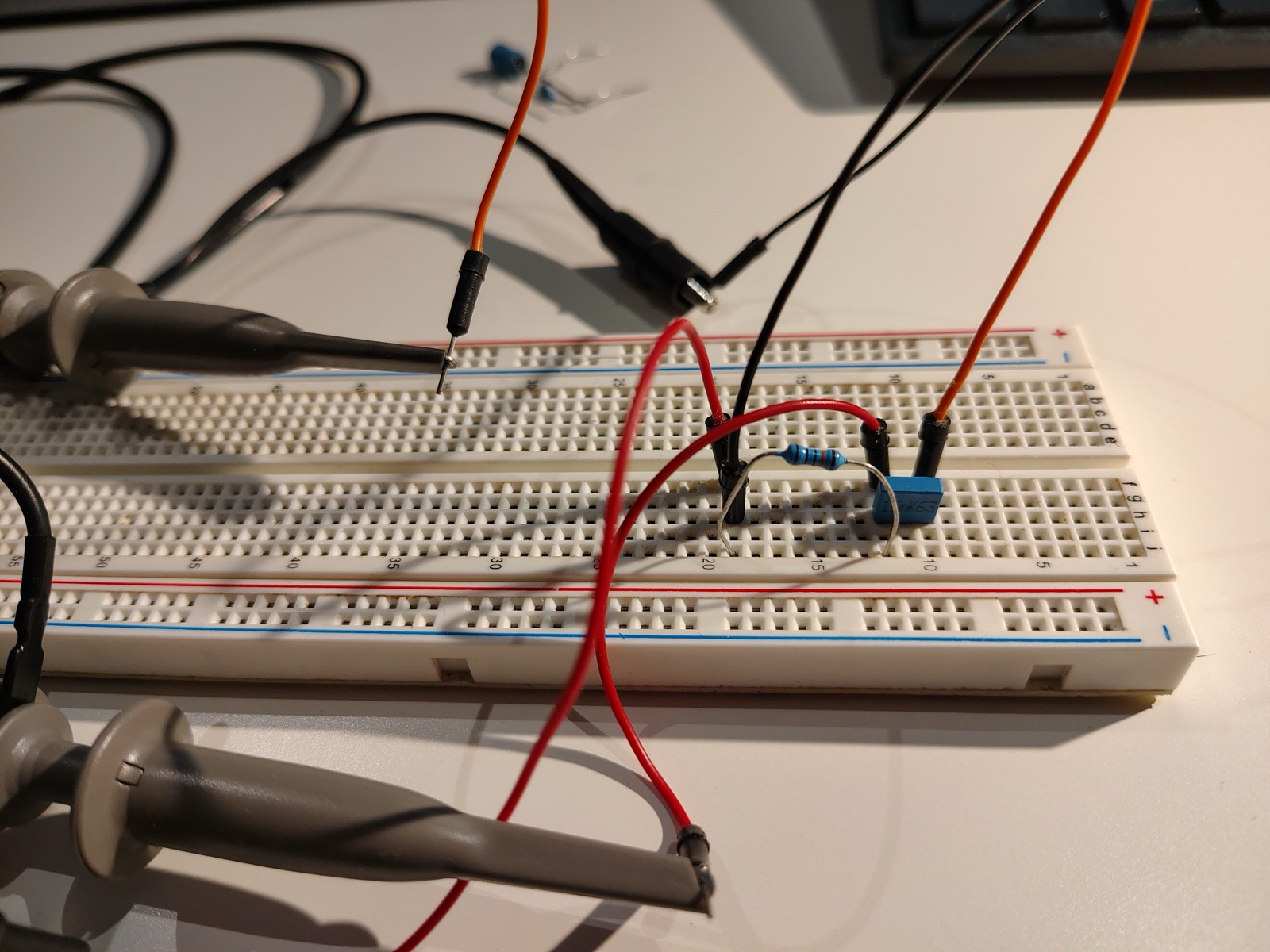
Figure L3.5. The series RC high-pass circuit on a breadboard (the same layout as in Lab 1).
Use the multimeter to measure the exact value of \(R_R\).
RC circuit resistance
Resistor resistance (\(R_R\)): \(\pm\) \(\mathrm{k\Omega }\) (measured with multimeter)
Set the oscilloscope to \(V_\text{max} = \pm1\,\mathrm{V}\) and the timescale to \(2\,\mathrm{ms}\)/div.
Set the generator waveform to “sine” and the amplitude to \(800\,\mathrm{m V}\).
Scan the frequency range from \(20\,\mathrm{Hz}\) to \(500\,\mathrm{Hz}\), noting \(V_\text{out}\) with the peak-to-peak measurement tool.
Record these readings in your notebook.
Focus on the region where \(V_\text{out}\) is \(1/\sqrt 2\) of its maximum value, and estimate the cutoff frequency \(f_c\).
Cutoff frequency
Cutoff frequency (\(f_c\)): \(\pm\) \(\mathrm{Hz}\) (at \(1/\sqrt{2}\) of max amplitude)
L3.5 Analysis and discussion
Show your derivations for all calculations. When computing an error for a derived quantity, use the rules in Error propagation in the Lab Guide.
Plot the RLC response curve using your readings of \(V_\text{out}\) as a function of frequency. How does the curve qualitatively compare to the theoretical curve of Figure L3.2?
Using the measured bandwidth \(\Delta f\) and resonant frequency \(f_0\) of the RLC response curve, as well as the capacitance of the \(\sim15\,\mathrm{n F}\) capacitor measured in Lab 1, compute the internal resistance of the Picoscope wave generator and the inductance of the inductor. Show your derivations and estimate your errors. Are the results what you would expect? Why or why not?
Using the period and amplitudes measured from the RLC ringdown curve, as well as the measured capacitance of the capacitor, compute the internal resistance of the Picoscope wave generator and the inductance of the inductor. Show your derivations and estimate your errors. Compare these results to those from the response curve. Explain any differences.
Plot the RC response curve using your readings of \(V_\text{out}\) as a function of frequency. How does the curve qualitatively compare to the theoretical curve of Figure L3.1?
Using the measured cutoff frequency \(f_c\) and the measured resistance of the resistor, determine the capacitance. Show your derivations and estimate your errors. Compare this with the value of the capacitance measured in Lab 1. Comment on any differences.
Bonus: estimate \(C\) using the slope of the response curve at low frequencies.
L3.6 Instructions for the lab report
Submit a lab report that includes:
A short Introduction giving background and context (e.g. explaining what filters are and how they are used) and explaining the goals of the experiment.
A Results section giving measured values, tables and plots.
An Analysis section showing how inferred (i.e. calculated) values are derived from measured ones.
A Discussion section commenting on sources of error and comparisons between different measurements.
A brief Conclusions section summarizing the results and placing them in context.